
Project Tracker Formatting That Shows Status
By Mark Fulton · 2026-09-14 · 12 min read
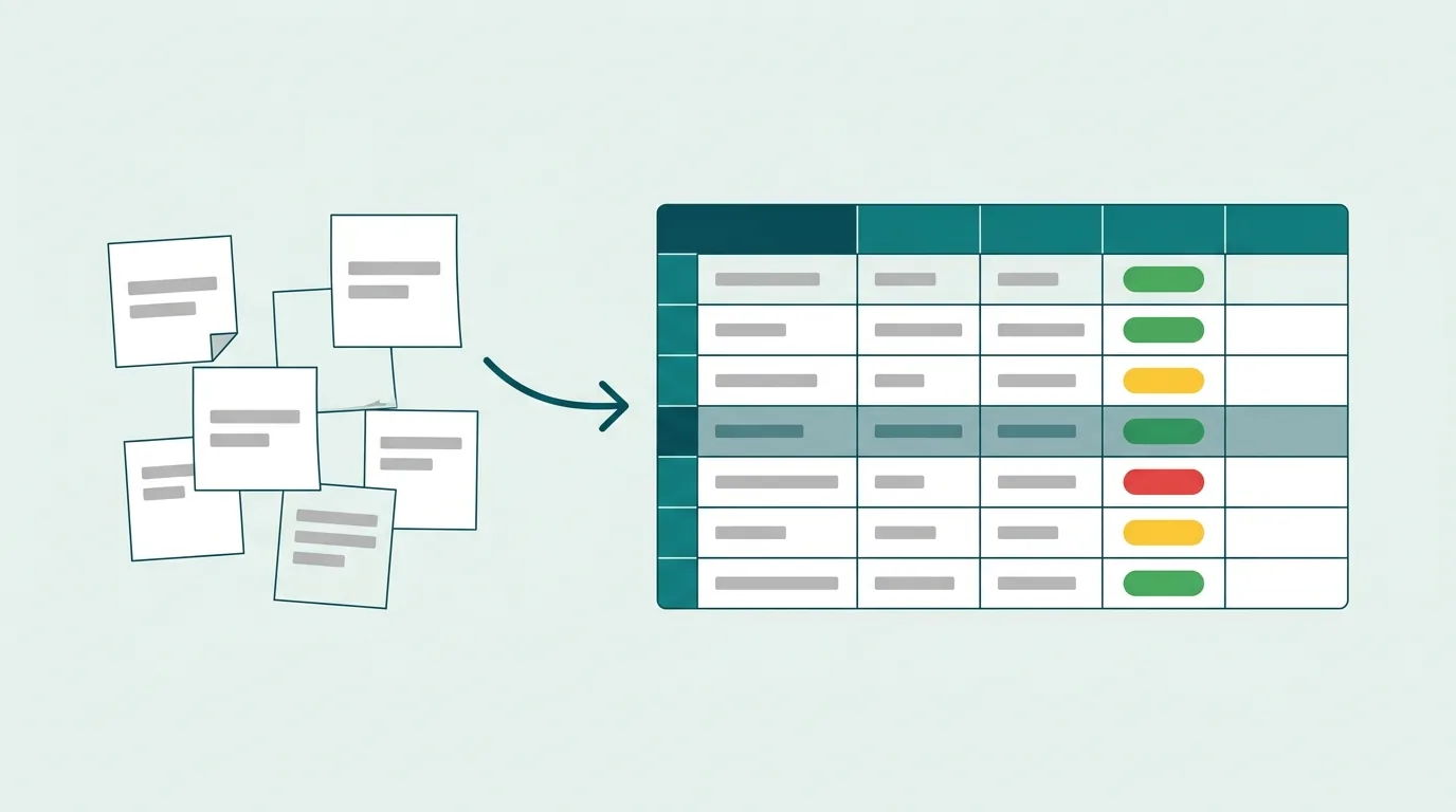
A project tracker spreadsheet reads well when its Status column can only hold a short, fixed list of values, set with data validation, so every "Done" is spelled the same way. With that in place the tracker needs two conditional formatting rules, not a rule per status: one that fades finished rows so open work stands out, and one that marks an overdue due date in bold dark red text on the date cell alone. Everything else, from RAG colours on every row to amber "due soon" fills, makes the sheet louder without making it clearer.
Search for a project tracker and you mostly get downloads. A template is a reasonable starting point, but it arrives with conditional formatting already wired in and no explanation of what each rule does, so the first time someone types "complete" instead of picking "Done", the colours quietly stop matching reality. The tracker most people actually have is one they built themselves, and it can be fixed in place.
Why do tracker columns drift into chaos?
Because the Status column is free text, and free text is typed by several people across several weeks. Each of them is right in their own head. "Done", "done", "Complete", a check-mark emoji and "Done" with a trailing space all mean the same thing to a human and are five different values to a spreadsheet.
Here is a nine-row tracker in exactly that state. It has six conditional formatting rules, each a "Cell Value equal to" rule on the Status column: green for Done, Complete and ✅, yellow for In progress and WIP, red for Blocked.
| A: Task | B: Owner | C: Due | D: Status | Renders as | |
|---|---|---|---|---|---|
| 2 | Draft launch brief | Priya | 2026-09-02 | Done | green row |
| 3 | Book venue | Sam | 9/5 | done | green row |
| 4 | Confirm catering | Sam | 2026-09-09 | Complete | green row |
| 5 | Design invitations | Leah | Sept 10 | ✅ | green row |
| 6 | Send invitations | Leah | 2026-09-12 | In progress | yellow row |
| 7 | Build RSVP form | Tom | ASAP | WIP | yellow row |
| 8 | Brief photographer | Priya | 2026-09-16 | blocked, waiting on budget | no colour |
| 9 | Print name badges | Tom | 2026-09-18 | Done |
no colour |
| 10 | Rehearsal run | Sam | 2026-09-19 | no colour |
Look at what the colours say. The one task that is actually stuck, row 8, is plain, because its status carries a note and no longer equals "Blocked". Row 9 is finished but looks untouched, because of one invisible space. Row 10 has no status at all. Three of the six rules exist only to catch spelling variants of one state, and the rule that matters most never fires.
The counting is worse. Five tasks are finished. =COUNTIF(D2:D10,"Done") returns 2: it catches rows 2 and 3, since COUNTIF ignores case, and misses "Complete", the emoji and the trailing space. Microsoft's own COUNTIF documentation warns that leading and trailing spaces return unexpected results, and this is what that looks like in practice.
The due dates have the same disease. "9/5", "Sept 10" and "ASAP" are not dates a formula can compare, so no overdue rule can ever see them.
How should a status column be constrained?
With a drop-down list that rejects anything else. Four values cover most trackers: Not started, In progress, Blocked, Done. Resist adding a fifth until someone can say what they would do differently for it. "On hold" and "Blocked" are usually the same instruction to the reader: this is not moving.
In Excel for Windows, select the Status cells (D2:D10 here), then go to Data → Data Validation. On the Settings tab, set Allow to List and type Not started,In progress,Blocked,Done into Source. Leave In-cell dropdown ticked. On the Error Alert tab, choose the Stop style so an off-list entry is refused rather than just warned about. On a Mac the command sits under Data, labelled Data Validation or Validate depending on version; in Excel for the web it is Data → Data Tools → Data Validation. The full walkthrough, including sourcing the list from a table on another sheet, is in Microsoft's guide to creating a drop-down list.
In Google Sheets, select the cells and use Insert → Dropdown, or Data → Data validation → Add rule, then pick Dropdown under Criteria and enter each option. Sheets rejects off-list input by default; the Advanced options let you downgrade that to a warning, which you should not do for a status column. Sheets also offers a preset "Project status" dropdown from the @ menu, which is fine as long as you trim its options to the four you mean.
Validation governs what gets entered from now on. It does not rewrite the values already sitting in the column, so clean those first: filter the Status column to see every distinct value, then replace "Complete", "✅" and "done" with "Done". Trailing spaces are the one you will not see in that filter list, so run TRIM over the column or use a tool that reports them.
How many conditional rules does a tracker need?
Two. Once the status vocabulary is fixed, colour stops having to decode spelling and can do its actual job: pointing at the rows that need someone.
Rule 1: fade what is finished. Select A2:E10 and add a formula rule:
=$D2="Done"
Format it with a mid-grey font, dark enough to still read. In Excel that is Home → Conditional Formatting → New Rule → Use a formula to determine which cells to format; in Sheets, Format → Conditional formatting, then Custom formula is under "Format cells if". The $ pins the test to column D, and the relative row lets each row check its own status. The formula is written for A2 because A2 is the top-left of the selection; select from row 1 by mistake and every row gets judged by the status of the row above it. The mechanics of relative references in rules are covered properly in conditional formatting that actually helps.
Why fade Done rather than colour the open states? Because in a live tracker most rows are either done or not yet urgent, and highlighting the majority turns colour into wallpaper. Greying out finished work does the opposite: the eye skips it and lands on everything still open.
What about Blocked? It does not need a fill. The word "Blocked" is already in the row, it is now spelled one way, and a filter on Status shows every blocked task in one click. That is also the version that survives being printed in greyscale.
How should dates signal overdue without shouting?
On the date cell only, with weight as well as colour. Select C2:C10 and add:
=AND($C2<>"",$C2<TODAY(),$D2<>"Done")
Format it as bold dark red text, no fill. Three conditions, each for a reason. $C2<>"" stops blank due dates from flagging, because an empty cell compares as zero and zero is earlier than today. $C2<TODAY() is the actual test, and TODAY() recalculates, so the rule stays current without anyone touching it. $D2<>"Done" stops finished work from nagging. Google's help page on custom formulas in conditional formatting shows the same row-anchored pattern, and the formula works unchanged in both apps.
The bold matters as much as the red. WCAG's Use of Color criterion is a Level A requirement that colour not be the only visual means of conveying information, and a spreadsheet read by a colleague with a colour vision deficiency is exactly the case it describes. Bold gives a second channel. If the tracker gets reviewed in meetings, add a third: a Days late column with =IF(AND(C2<>"",D2<>"Done",C2<TODAY()),TODAY()-C2,""), which shows a number you can sort by.
What to leave out: an amber "due this week" band. It fires on a large share of open rows at any given moment, which means it fires on the rows people are already working on.
Here is the same tracker after the cleanup, viewed on 14 September 2026:
| A: Task | B: Owner | C: Due | D: Status | E: Notes | Renders as | |
|---|---|---|---|---|---|---|
| 2 | Draft launch brief | Priya | 2026-09-02 | Done | grey text | |
| 3 | Book venue | Sam | 2026-09-05 | Done | grey text | |
| 4 | Confirm catering | Sam | 2026-09-09 | Done | grey text | |
| 5 | Design invitations | Leah | 2026-09-10 | Done | grey text | |
| 6 | Send invitations | Leah | 2026-09-12 | In progress | due date bold dark red | |
| 7 | Build RSVP form | Tom | 2026-09-11 | In progress | Date agreed with Tom | due date bold dark red |
| 8 | Brief photographer | Priya | 2026-09-16 | Blocked | Waiting on budget | plain |
| 9 | Print name badges | Tom | 2026-09-18 | Done | grey text | |
| 10 | Rehearsal run | Sam | 2026-09-19 | Not started | plain |
Six rules became one, plus one for dates. The note that was hiding inside row 8's status moved to its own column, "ASAP" became a real date (which took a question to Tom, not a formula), and COUNTIF(D2:D10,"Done") now returns 5. The two rows in dark red are the only two that are both open and late, and nothing else on the sheet competes with them. If the text dates in your own tracker will not convert cleanly, fixing inconsistent dates in Excel walks through why and how.
What belongs in a tracker and what belongs elsewhere?
A tracker is one row per task and one fact per column: task, owner, due date, status, and a notes column so that commentary never leaks into the status. Priority is worth a column only if it changes the order people work in. A percent-complete column next to Status usually tells the same story twice and eventually tells two different ones.
Some things are better on their own tab:
- The list of allowed statuses, if you source the drop-down from a range rather than typing it in. Microsoft recommends keeping it in a table so the drop-down updates when the list does.
- The project-level RAG status. Red, amber or green describes the project, not each task, so it belongs in a small summary block, not coloured across 60 rows.
- Counts by status, one
COUNTIFper value, above the table or on a summary tab. - Budget, risks and meeting notes. Each has its own shape, and bolting them onto task rows is how trackers grow blank spacer rows and merged headers.
How do you keep it readable at 200 rows?
The two rules above scale; the habits around them are what break.
Apply each rule once to the whole data range. In Excel, copying cells, filling down or using Format Painter creates a new rule for the destination cells, and Google Sheets carries rules along when you paste too. A tracker that is edited for a few months ends up with dozens of copies of the same rule over fragments of rows. Open Manage Rules, set the scope to This Worksheet, delete the duplicates and reapply one rule to the full range.
Make it a real Excel table with Ctrl+T, so the range expands to include each new row you add instead of stopping at the last row you happened to format.
Freeze the header row and sort by due date, so the late rows gather together rather than hiding on page four. The header and width basics are in the seven rules for a professional-looking sheet, and the table layout rules behind them are in Excel table design best practices.
Filter instead of colouring. At 200 rows nobody scans for yellow. They filter Status to "Blocked" or sort by Days late. A consistent status column is what makes that filter trustworthy.
Move finished work out once a phase closes. A Done tab keeps history intact and keeps the live tracker short enough to read on one screen.
Frequently asked questions
How do I make a dropdown status column in Excel?
Select the Status cells, go to Data → Data Validation, set Allow to List, and type your values separated by commas in Source, for example Not started,In progress,Blocked,Done. On the Error Alert tab choose Stop so anything off the list is refused. On a Mac look for Data Validation or Validate under the Data tab; in Excel for the web it is under Data → Data Tools. Clean the existing values first, since validation does not change what is already there.
Should overdue tasks be red?
Red text on the due date, yes. A red fill across the whole row, usually no: it overwhelms the row's other information and, repeated on several rows, reads as a wall of alarm. Pair the colour with bold or a Days late number, so the signal still works for readers who do not see red clearly and on a greyscale printout.
How do I count tasks by status?
Use COUNTIF with the status as the criteria, anchoring the range so the formula can be copied: =COUNTIF($D$2:$D$200,"Blocked"). COUNTIF is not case sensitive, but it does treat "Done " with a trailing space and "Complete" as different values, which is why the count is only reliable once the column is a drop-down.
Why do my conditional formatting rules multiply?
Copy and paste, filling a range and Format Painter each create a new rule for the destination cells, so a sheet that gets edited for a while collects copies of the same rule over small fragments of the range. The fix is to open Home → Conditional Formatting → Manage Rules, switch the scope to This Worksheet, delete the fragments, and apply a single rule to the full data range. New rules also go to the top of the list and take precedence, so check the order while you are there.
Try it on your own tracker
Drop your tracker into the Excel formatter and it proposes a plan before touching anything: cleaned-up header text, proper date formats, a frozen header row, and, where it finds them, trimmed stray spaces, the kind that turn "Done " into a status of its own. Each change is listed so you approve it, and the result downloads as a new .xlsx while the original stays as it was. It will not invent your status vocabulary or restructure a tab that holds more than one table, because those are decisions only the person running the project can make. Add the drop-down and the two rules above to the formatted file and you have a tracker that says what state the work is in.